本文系统分析 Kaggle Home Credit Default Risk 竞赛方案,介绍从数据预处理、特征工程到模型集成的完整机器学习流程。文章讨论该大规模信用风险预测任务中的架构选择、实现策略与性能优化方法,涵盖数据质量评估、关系型数据库的特征提取、梯度提升模型优化和堆叠集成,为类似金融风险结构化数据预测任务提供实践参考。
关键词#
信用风险建模、梯度提升、特征工程、模型堆叠、LightGBM、XGBoost、CatBoost、机器学习流水线
1. 引言与业务背景#
1.1 问题领域与研究动机#
金融服务普及已成为全球经济发展的重要挑战。传统信用评估高度依赖既有信用记录、稳定就业记录和可抵押资产;按照世界银行 2017 年全球普惠金融数据库的统计,全球约有 17 亿成年人无法获得正规银行服务,这些标准使他们难以进入传统信贷体系。
Home Credit Group 是一家在 10 多个国家开展业务的国际非银行金融机构,主要服务缺乏既有信用记录、通常被传统银行拒绝的“信用不可见”人群。核心业务挑战是利用替代数据,在约 5 分钟的有限时间内完成准确的违约预测。
1.2 信用风险预测任务#
任务定义:预测违约概率(PD)的二分类问题。
\[
Y_i = \begin{cases}
1, & \text{if client } i \text{ defaults (90+ days past due)} \\\\
0, & \text{if client } i \text{ repays as scheduled}
\end{cases}
\]
评价指标:受试者工作特征曲线下面积(ROC-AUC)。
选择 AUC,是因为它对类别不平衡相对稳健,重点衡量排序能力,而非绝对概率的校准程度:
\[
\text{AUC} = \int_0^1 \text{TPR}(\tau) \, d(\text{FPR}(\tau))
\]
其中,\(\text{TPR}\) 表示真正率,\(\text{FPR}\) 表示阈值 \(\tau\) 下的假正率。
指标解读:
- AUC = 0.50:随机预测,没有区分能力。
- AUC ∈ [0.60, 0.70]:表现较差。
- AUC ∈ [0.70, 0.80]:表现可接受。
- AUC ∈ [0.80, 0.90]:表现良好。
- AUC > 0.90:表现优秀,但需要核查过拟合。
1.3 信用评估中的替代数据#
该竞赛数据集体现了向替代信用评分转变的思路,涉及非传统数据形态:
| 传统数据 | 替代性代理数据 | 数据提供方 |
|---|
| 信用评分 | 手机充值模式、通话时长 | 电信运营商 |
| 收入证明 | POS 交易记录、租金支付历史 | 支付机构、房产平台 |
| 银行流水 | 分期还款历史、信用卡账单 | 消费金融公司 |
| 就业证明 | 电商活动、社交媒体互动 | 互联网平台 |
1.4 竞赛成果与方法影响#
2018 年 Home Credit Default Risk 竞赛吸引了全球 7,194 支队伍。优秀方案体现了以下方法创新:
- 特征工程:从基础聚合发展到时间窗口特征和趋势分析。
- 集成架构:系统应用多层堆叠策略。
- 数据预处理:改进缺失值填补与异常值处理。
这些方法也已应用于保险欺诈检测、营销响应预测和客户流失建模等相关领域。
2. 数据集架构与表结构分析#
2.1 数据规模与关联结构#
数据集由七张相互关联的关系表组成,总记录数超过 5,000 万,体现了企业金融系统常见的复杂关系型数据库结构。
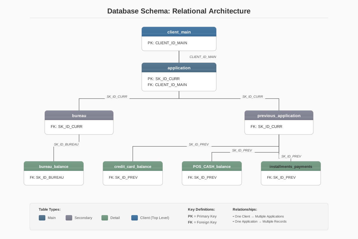
数据表统计概览:
| 数据表 | 行数 | 存储大小 | 说明 | 主键 | 外键 |
|---|
| application_{train,test} | 307,511 / 48,744 | 45MB / 7MB | 主申请表 | SK_ID_CURR | — |
| bureau | 1,716,428 | 172MB | 征信记录 | SK_ID_BUREAU | SK_ID_CURR |
| bureau_balance | 27,299,925 | 574MB | 每月征信状态 | — | SK_ID_BUREAU |
| previous_application | 1,670,214 | 150MB | 历史申请 | SK_ID_PREV | SK_ID_CURR |
| installments_payments | 13,605,401 | 730MB | 分期还款记录 | — | SK_ID_PREV |
| POS_CASH_balance | 10,001,358 | 970MB | POS 现金贷款账单 | — | SK_ID_PREV |
| credit_card_balance | 3,840,312 | 400MB | 信用卡账单 | — | SK_ID_PREV |
2.2 实体关系模型#
数据库采用分层关联结构,包含三个主要标识符域:
1
2
3
| SK_ID_CURR: Client-level identifier (primary entity key)
SK_ID_PREV: Previous application identifier (transaction-level)
SK_ID_BUREAU: External credit bureau record identifier
|
关系拓扑:
1
2
3
4
5
6
| application [1] ───<N>─── bureau [1] ───<N>─── bureau_balance
│
├─<N>─── previous_application [1] ───<N>─── installments_payments
│ ├─<N>─── POS_CASH_balance
│ └─<N>─── credit_card_balance
└─<N>─── credit_card_balance
|
一对多(1:N)关系要求在特征工程中进行聚合,将时间序列和多条记录转换为机器学习模型可用的静态特征向量。
2.3 字段详解#
2.3.1 申请表:主实体#
申请表是核心实体,训练集部分包含目标标签。
人口统计与申请特征:
 1
 2
 3
 4
 5
 6
 7
 8
 9
10
| SK_ID_CURR: Integer (primary identifier)
TARGET: Binary (0=non-default, 1=default) - training set only
CODE_GENDER: Categorical (M/F/XNA)
FLAG_OWN_CAR: Binary (Y/N)
FLAG_OWN_REALTY: Binary (Y/N)
CNT_CHILDREN: Integer (count of children)
AMT_INCOME_TOTAL: Float (annual income in local currency)
AMT_CREDIT: Float (loan amount requested)
AMT_ANNUITY: Float (monthly installment amount)
AMT_GOODS_PRICE: Float (price of goods being financed)
|
时间特征:以相对申请日期的天数编码,负值表示过去。
1
2
3
4
5
| DAYS_BIRTH: Integer (age in days, e.g., -10000 ≈ 27.4 years)
DAYS_EMPLOYED: Integer (employment duration, special value 365243 indicates unemployed)
DAYS_REGISTRATION: Integer (registration change recency)
DAYS_ID_PUBLISH: Integer (identity document issuance recency)
DAYS_LAST_PHONE_CHANGE: Integer (mobile phone change recency)
|
外部评分特征:具有较强预测能力的归一化评分。
1
2
3
4
| EXT_SOURCE_1: Float [0,1] (normalized external score 1)
EXT_SOURCE_2: Float [0,1] (normalized external score 2)
EXT_SOURCE_3: Float [0,1] (normalized external score 3)
# Sourced from third-party credit bureaus
|
2.3.2 征信表:外部信用历史#
记录客户与外部金融机构之间的信贷关系。
 1
 2
 3
 4
 5
 6
 7
 8
 9
10
11
12
13
14
15
16
17
| SK_ID_CURR: Integer (foreign key to application)
SK_ID_BUREAU: Integer (unique bureau record identifier)
CREDIT_ACTIVE: Categorical (Active/Closed/Sold/Demand/Bad debt)
CREDIT_CURRENCY: Categorical (currency code)
DAYS_CREDIT: Integer (days since credit application)
CREDIT_DAY_OVERDUE: Integer (current days past due)
DAYS_CREDIT_ENDDATE: Integer (remaining duration to maturity)
DAYS_ENDDATE_FACT: Integer (actual closure date)
AMT_CREDIT_MAX_OVERDUE: Float (maximum historical overdue amount)
CNT_CREDIT_PROLONG: Integer (count of credit prolongations)
AMT_CREDIT_SUM: Float (total credit exposure)
AMT_CREDIT_SUM_DEBT: Float (outstanding debt)
AMT_CREDIT_SUM_LIMIT: Float (credit limit)
AMT_CREDIT_SUM_OVERDUE: Float (current overdue amount)
CREDIT_TYPE: Categorical (loan type: consumer, mortgage, etc.)
DAYS_CREDIT_UPDATE: Integer (recency of bureau update)
AMT_ANNUITY: Float (monthly payment obligation)
|
2.3.3 征信月度余额表:征信状态变化#
每条征信记录的月度状态快照,可用于趋势分析。
 1
 2
 3
 4
 5
 6
 7
 8
 9
10
11
| SK_ID_BUREAU: Integer (foreign key to bureau)
MONTHS_BALANCE: Integer (relative month index, -1=last month, -2=two months ago)
STATUS: Categorical encoding:
'0': Current (no delinquency)
'1': 1-29 days past due
'2': 30-59 days past due
'3': 60-89 days past due
'4': 90-119 days past due
'5': 120-149 days past due
'C': Closed (paid off)
'X': Status unknown
|
2.3.4 历史申请表#
Home Credit 系统内部的历史申请。
 1
 2
 3
 4
 5
 6
 7
 8
 9
10
11
12
13
14
15
| SK_ID_CURR: Integer (foreign key)
SK_ID_PREV: Integer (unique previous application identifier)
NAME_CONTRACT_TYPE: Categorical (Cash/Consumer/Revolving loans)
AMT_ANNUITY: Float (proposed monthly payment)
AMT_APPLICATION: Float (requested amount)
AMT_CREDIT: Float (approved amount)
AMT_DOWN_PAYMENT: Float (down payment amount)
RATE_DOWN_PAYMENT: Float (down payment ratio)
RATE_INTEREST_PRIMARY: Float (primary interest rate)
RATE_INTEREST_PRIVILEGED: Float (preferential interest rate)
NAME_CONTRACT_STATUS: Categorical (Approved/Refused/Canceled/Unused)
DAYS_DECISION: Integer (days since decision)
CODE_REJECT_REASON: Categorical (rejection reason if applicable)
NAME_CLIENT_TYPE: Categorical (New/Repeat customer)
CNT_PAYMENT: Integer (proposed term in months)
|
2.3.5 分期还款表#
细粒度还款交易记录。
1
2
3
4
5
6
7
8
| SK_ID_CURR: Integer (foreign key)
SK_ID_PREV: Integer (foreign key to previous_application)
NUM_INSTALMENT_VERSION: Integer (version of installment schedule)
NUM_INSTALMENT_NUMBER: Integer (installment sequence number)
DAYS_INSTALMENT: Integer (scheduled payment date)
DAYS_ENTRY_PAYMENT: Integer (actual payment date)
AMT_INSTALMENT: Float (scheduled amount)
AMT_PAYMENT: Float (actual amount paid)
|
衍生指标:
- 逾期天数(DPD):\(DPD = DAYS_ENTRY_PAYMENT - DAYS_INSTALMENT\)
- 还款金额偏差:\(\Delta AMT = AMT_PAYMENT - AMT_INSTALMENT\)
2.4 数据质量概况#
类别分布:
1
2
3
| Class 0 (Non-default): 282,686 observations (91.93%)
Class 1 (Default): 24,825 observations (8.07%)
Imbalance Ratio: 11.4:1
|
缺失值概览:
- EXT_SOURCE_1:缺失率 56.38%。
- EXT_SOURCE_3:缺失率 19.83%。
- AMT_ANNUITY:缺失率 0.003%。
- OCCUPATION_TYPE:缺失率 31.35%。
异常编码:
- DAYS_EMPLOYED = 365,243(约 1,000 年):表示失业的哨兵值。
- CODE_GENDER = ‘XNA’:未指定的性别类别。
- AMT_INCOME_TOTAL:出现 117,000,000 的极端值,可能是数据错误。
3. 系统架构与流水线设计#
3.1 框架选择:Steppy 流水线架构#
方案采用 Steppy,这是面向模块化、可复现数据科学流程的轻量级机器学习流水线库。Steppy 借鉴 Apache Airflow、Spotify Luigi 等工作流编排系统的设计原则,并针对机器学习任务进行适配。
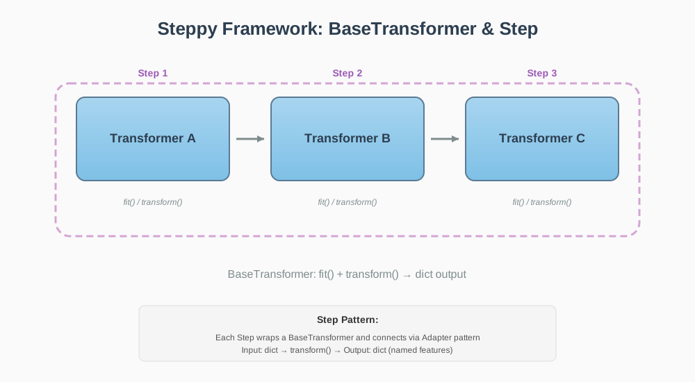
使用流水线框架的原因:
传统命令式机器学习代码存在以下架构局限:
1
2
3
4
5
6
7
| # Anti-pattern: Tightly coupled workflow
data = load_data()
data = clean_data(data)
data = extract_features(data)
X_train, X_test, y_train, y_test = split_data(data)
model = train_model(X_train, y_train)
predictions = model.predict(X_test)
|
主要不足:
- 耦合:修改某个阶段,需要理解下游依赖。
- 可复现性:中间结果难以缓存或进行版本管理。
- 并行化:顺序执行限制了计算资源优化。
- 实验追踪:难以系统比较不同参数配置。
Steppy 的声明式方法:
 1
 2
 3
 4
 5
 6
 7
 8
 9
10
11
12
13
14
15
16
17
18
19
20
21
22
23
24
25
26
27
| from steppy.base import BaseTransformer
class DataLoader(BaseTransformer):
"""Loads raw data from persistent storage."""
def transform(self, filepath):
data = pd.read_csv(filepath)
return {'data': data}
class DataCleaningTransformer(BaseTransformer):
"""Applies data quality transformations."""
def transform(self, data):
cleaned = self._handle_outliers(data)
cleaned = self._impute_missing(cleaned)
return {'cleaned_data': cleaned}
def _handle_outliers(self, df):
# Implementation
pass
class FeatureExtractionTransformer(BaseTransformer):
"""Engineers features from cleaned data."""
def transform(self, cleaned_data):
features = self._aggregate_features(cleaned_data)
return {'features': features}
|
设计原则:
- 标准接口:所有组件继承
BaseTransformer,提供 fit() 和 transform() 方法。 - 显式数据流:使用带命名键的字典传递输入输出,便于追踪。
- 可组合性:通过
Step 和 Adapter 抽象连接各步骤。 - 持久化:中间产物支持缓存与检查点。
3.2 端到端流水线#
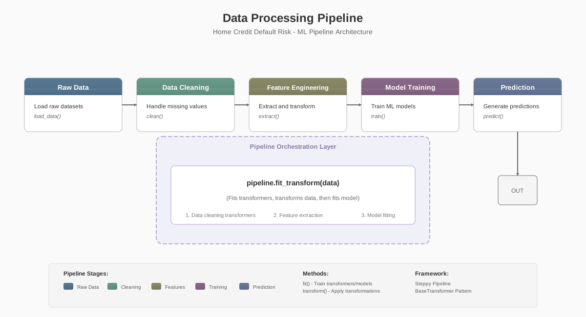
阶段 1:数据读取与清洗
 1
 2
 3
 4
 5
 6
 7
 8
 9
10
11
12
13
14
15
16
17
18
19
20
21
22
23
| def build_data_ingestion_pipeline(config):
"""Constructs the data loading and cleaning pipeline stage."""
# Load all seven tables
raw_data = DataLoader(config.data_paths).transform()
# Apply table-specific cleaning transformers
cleaning_transformers = {
'application': ApplicationCleaning(),
'bureau': BureauCleaning(),
'bureau_balance': BureauBalanceCleaning(),
'previous_application': PreviousApplicationCleaning(),
'installments_payments': InstallmentPaymentsCleaning(),
'pos_cash_balance': PosCashBalanceCleaning(),
'credit_card_balance': CreditCardBalanceCleaning()
}
cleaned_data = {
table: transformer.transform(raw_data[table])
for table, transformer in cleaning_transformers.items()
}
return cleaned_data
|
阶段 2:特征工程
 1
 2
 3
 4
 5
 6
 7
 8
 9
10
11
12
13
14
15
16
17
18
19
20
21
22
23
24
25
26
27
28
29
30
31
32
33
34
35
36
| def build_feature_engineering_pipeline(cleaned_data):
"""Constructs the feature extraction pipeline stage."""
# Table-specific feature extraction
bureau_features = BureauFeatureExtractor().transform(
cleaned_data['bureau'],
cleaned_data['bureau_balance']
)
prev_app_features = PreviousApplicationFeatureExtractor().transform(
cleaned_data['previous_application']
)
installment_features = InstallmentFeatureExtractor().transform(
cleaned_data['installments_payments']
)
# Feature consolidation
all_features = FeatureConcatenator().transform([
cleaned_data['application'],
bureau_features,
prev_app_features,
installment_features
])
# Categorical encoding
encoded_features = CategoricalEncoder().transform(
all_features,
method='target_encoding'
)
return {
'features': encoded_features,
'target': cleaned_data['application']['TARGET'],
'feature_names': encoded_features.columns.tolist()
}
|
阶段 3:模型训练
 1
 2
 3
 4
 5
 6
 7
 8
 9
10
11
12
13
14
15
16
17
18
19
20
21
22
23
24
| def build_model_training_pipeline(feature_data, config):
"""Constructs the model training pipeline stage."""
# Train/validation split
X_train, X_valid, y_train, y_valid = train_test_split(
feature_data['features'],
feature_data['target'],
test_size=0.2,
stratify=feature_data['target'],
random_state=config.random_seed
)
# Model initialization and training
model = GradientBoostingModel(config.model_params)
model.fit(X_train, y_train, validation_data=(X_valid, y_valid))
# Performance evaluation
validation_auc = roc_auc_score(y_valid, model.predict(X_valid))
return {
'model': model,
'validation_auc': validation_auc,
'feature_importance': model.feature_importances_
}
|
阶段 4:构建堆叠集成(Stacking)
 1
 2
 3
 4
 5
 6
 7
 8
 9
10
11
12
13
14
15
16
17
18
19
20
21
22
23
24
25
26
27
28
29
30
31
32
33
| def build_stacking_ensemble(base_models, meta_learner, X, y, X_test):
"""
Implements two-level stacking ensemble architecture.
Level 1: Base learners generate out-of-fold predictions
Level 2: Meta-learner trains on base model outputs
"""
# Generate OOF predictions
oof_predictions = {}
test_predictions = {}
for name, model in base_models.items():
oof_pred, test_pred = generate_oof_predictions(
model, X, y, X_test, n_folds=5
)
oof_predictions[name] = oof_pred
test_predictions[name] = test_pred
# Train meta-learner
meta_features = np.column_stack([
oof_predictions[name] for name in base_models.keys()
])
meta_learner.fit(meta_features, y)
# Generate final predictions
meta_test_features = np.column_stack([
test_predictions[name] for name in base_models.keys()
])
final_predictions = meta_learner.predict_proba(meta_test_features)[:, 1]
return final_predictions
|
3.3 项目目录组织#
 1
 2
 3
 4
 5
 6
 7
 8
 9
10
11
12
13
14
15
16
17
18
19
20
21
22
23
24
25
| open-solution-home-credit/
├── src/ # Source code modules
│ ├── __init__.py
│ ├── pipeline_manager.py # Orchestration layer
│ ├── pipelines.py # Pipeline definitions (9 model configurations)
│ ├── pipeline_blocks.py # Step factory methods
│ ├── feature_extraction.py # Feature transformers (20+ implementations)
│ ├── data_cleaning.py # Data quality transformers (7 table-specific)
│ ├── models.py # Model wrappers (LGB/XGB/CTB/NN/RF/LR)
│ ├── pipeline_config.py # Configuration constants and hyperparameters
│ ├── hyperparameter_tuning.py # Optimization strategies
│ ├── callbacks.py # Training monitoring callbacks
│ ├── utils.py # Utility functions
│ └── neptune_hacks.py # Offline experiment tracking support
├── configs/ # Configuration files
│ └── neptune.yaml # Main configuration (paths/hyperparameters)
├── data/ # Data directory
│ ├── raw/ # Original competition data
│ └── workdir/ # Intermediate processing artifacts
├── notebooks/ # Exploratory data analysis
├── blog/ # Documentation
│ └── images/ # Visualization assets
├── main.py # CLI entry point
├── requirements.txt # Dependency specification
└── README.md # Project documentation
|
3.4 配置管理#
项目采用混合配置策略:YAML 管理实验参数,Python 模块管理代码级常量。
实验配置(configs/neptune.yaml):
 1
 2
 3
 4
 5
 6
 7
 8
 9
10
11
12
13
14
15
16
17
18
19
20
21
22
23
24
25
26
27
28
29
30
31
32
33
34
35
| parameters:
# Data paths
train_filepath: /data/application_train.csv
test_filepath: /data/application_test.csv
# Model selection
pipeline_name: lightGBM
# Feature toggles
use_application: true
use_bureau: true
use_bureau_balance: true
use_previous_application: true
use_installments_payments: true
use_pos_cash_balance: true
use_credit_card_balance: true
# LightGBM hyperparameters
lgbm__objective: binary
lgbm__metric: auc
lgbm__num_leaves: 35
lgbm__learning_rate: 0.02
lgbm__n_estimators: 5000
lgbm__min_child_samples: 70
lgbm__subsample: 1.0
lgbm__colsample_bytree: 0.03
lgbm__reg_lambda: 100.0
lgbm__reg_alpha: 0.0
# Cross-validation configuration
n_cv_splits: 5
validation_size: 0.2
stratified_cv: true
shuffle: true
random_seed: 90210
|
代码级配置(src/pipeline_config.py):
 1
 2
 3
 4
 5
 6
 7
 8
 9
10
11
12
13
14
15
16
17
18
19
20
21
22
23
24
25
26
27
28
29
30
31
32
33
34
35
36
37
38
39
40
41
42
43
44
45
46
| """Constants and aggregation recipes for feature engineering."""
import numpy as np
# Reproducibility constants
RANDOM_SEED = 90210
DEV_SAMPLE_SIZE = 1000
# Column type definitions
CATEGORICAL_COLUMNS = [
'CODE_GENDER', 'FLAG_OWN_CAR', 'FLAG_OWN_REALTY',
'NAME_TYPE_SUITE', 'NAME_INCOME_TYPE', 'NAME_EDUCATION_TYPE',
'NAME_FAMILY_STATUS', 'NAME_HOUSING_TYPE', 'OCCUPATION_TYPE',
'WEEKDAY_APPR_PROCESS_START', 'ORGANIZATION_TYPE', 'FONDKAPREMONT_MODE',
'HOUSETYPE_MODE', 'WALLSMATERIAL_MODE', 'EMERGENCYSTATE_MODE'
]
NUMERICAL_COLUMNS = [
'AMT_INCOME_TOTAL', 'AMT_CREDIT', 'AMT_ANNUITY', 'AMT_GOODS_PRICE',
'DAYS_BIRTH', 'DAYS_EMPLOYED', 'DAYS_REGISTRATION', 'DAYS_ID_PUBLISH',
'EXT_SOURCE_1', 'EXT_SOURCE_2', 'EXT_SOURCE_3'
]
# Aggregation recipes for feature extraction
BUREAU_AGGREGATION_RECIPES = [
(['SK_ID_CURR'], [
('SK_ID_BUREAU', 'count'),
('AMT_CREDIT_SUM', ['sum', 'mean', 'max', 'std']),
('AMT_CREDIT_SUM_DEBT', ['sum', 'mean']),
('AMT_CREDIT_SUM_OVERDUE', ['sum', 'mean', 'max']),
('DAYS_CREDIT', ['min', 'max', 'mean']),
('CREDIT_DAY_OVERDUE', ['sum', 'max', 'mean']),
('CNT_CREDIT_PROLONG', 'sum')
])
]
PREVIOUS_APPLICATION_AGGREGATION_RECIPES = [
(['SK_ID_CURR'], [
('SK_ID_PREV', 'count'),
('AMT_APPLICATION', ['sum', 'mean', 'max']),
('AMT_CREDIT', ['sum', 'mean', 'max']),
('AMT_DOWN_PAYMENT', ['sum', 'mean']),
('RATE_INTEREST_PRIMARY', ['mean', 'max']),
('DAYS_DECISION', ['min', 'max', 'mean'])
])
]
|
这种配置分工带来以下特点:
- 易用性:通过 YAML 快速调整实验,无需修改代码。
- 类型安全:Python 模块提供编译阶段校验。
- 覆盖能力:支持命令行和环境变量覆盖配置。
4. 探索性数据分析与质量评估#
4.1 EDA 方法框架#
这里的探索性数据分析(EDA)围绕五个基本问题展开:
- 数据质量:有哪些异常、缺失值或编码不一致?
- 分布特征:各特征的集中趋势、离散程度与分布形态如何?
- 业务洞察:不同人群是否表现出不同的行为?
- 预测信号:哪些特征与目标变量存在统计关联?
- 特征工程方向:哪些变换或聚合可能提高预测能力?
4.2 关键发现#
4.2.1 类别不平衡分析#
 1
 2
 3
 4
 5
 6
 7
 8
 9
10
11
12
13
14
15
16
17
18
19
20
21
22
23
24
| import pandas as pd
import matplotlib.pyplot as plt
import seaborn as sns
# Load training data
train_df = pd.read_csv('data/application_train.csv')
# Class distribution analysis
target_distribution = train_df['TARGET'].value_counts()
print("Class Distribution:")
print(target_distribution)
print(f"\nClass Proportions:")
print(train_df['TARGET'].value_counts(normalize=True))
# Output:
# Class Distribution:
# 0 282686
# 1 24825
# Name: TARGET, dtype: int64
#
# Class Proportions:
# 0 0.919271
# 1 0.080729
# Name: TARGET, dtype: float64
|
解读:11.4:1 的类别比例要求谨慎选择指标。仅预测多数类就能达到 91.9% 的准确率,因此准确率可能产生误导,应结合 AUC 和精确率—召回率指标。
4.2.2 外部评分的预测能力#
 1
 2
 3
 4
 5
 6
 7
 8
 9
10
11
12
13
14
15
16
17
18
19
20
21
22
23
24
| # Analyze EXT_SOURCE features
fig, axes = plt.subplots(1, 3, figsize=(18, 5))
for idx, col in enumerate(['EXT_SOURCE_1', 'EXT_SOURCE_2', 'EXT_SOURCE_3']):
# Distribution comparison
sns.kdeplot(
data=train_df[train_df['TARGET'] == 0][col].dropna(),
label='Non-default',
ax=axes[idx],
fill=True,
alpha=0.5
)
sns.kdeplot(
data=train_df[train_df['TARGET'] == 1][col].dropna(),
label='Default',
ax=axes[idx],
fill=True,
alpha=0.5
)
axes[idx].set_title(f'{col} Distribution by Target')
axes[idx].legend()
plt.tight_layout()
plt.savefig('images/ext_source_kde.png', dpi=150)
|
主要观察:
- 违约客户的外部评分普遍更低。
- EXT_SOURCE_1 的区分能力最强,信息值(IV)最高。
- 缺失率存在差异:EXT_SOURCE_1 为 56.4%,EXT_SOURCE_2 为 0.2%,EXT_SOURCE_3 为 19.8%。
4.2.3 收入分布分析#
 1
 2
 3
 4
 5
 6
 7
 8
 9
10
| # Income distribution with log transformation
train_df['AMT_INCOME_TOTAL_LOG'] = np.log1p(train_df['AMT_INCOME_TOTAL'])
# Descriptive statistics
print(train_df['AMT_INCOME_TOTAL'].describe())
# Detect extreme outliers
q99 = train_df['AMT_INCOME_TOTAL'].quantile(0.99)
extreme_outliers = train_df[train_df['AMT_INCOME_TOTAL'] > q99 * 10]
print(f"\nExtreme outliers (>10x 99th percentile): {len(extreme_outliers)}")
|
统计概览:
1
2
3
4
5
6
7
8
| count 3.075110e+05
mean 1.687979e+05
std 2.371894e+05
min 2.565000e+04
25% 1.125000e+05
50% 1.471500e+05
75% 2.025000e+05
max 1.170000e+08 # Data quality concern
|
启示:分布明显右偏,偏度约为 3.2,适合考虑对数变换。最大值为 117M,而均值为 168K,这种极端差异提示可能存在需要处理的录入错误。
4.2.4 时间特征分析:年龄与违约风险#
 1
 2
 3
 4
 5
 6
 7
 8
 9
10
11
12
13
14
15
16
17
18
19
20
21
22
23
| # Age calculation and risk profiling
train_df['AGE_YEARS'] = -train_df['DAYS_BIRTH'] / 365.25
# Binned analysis
train_df['AGE_BIN'] = pd.cut(
train_df['AGE_YEARS'],
bins=[0, 25, 30, 35, 40, 45, 50, 60, 100],
labels=['<25', '25-30', '30-35', '35-40', '40-45', '45-50', '50-60', '60+']
)
default_by_age = train_df.groupby('AGE_BIN')['TARGET'].agg(['mean', 'count'])
print(default_by_age)
# Visualization
plt.figure(figsize=(10, 6))
default_by_age['mean'].plot(kind='bar', color='steelblue')
plt.title('Default Rate by Age Cohort')
plt.xlabel('Age Group')
plt.ylabel('Default Rate')
plt.axhline(y=train_df['TARGET'].mean(), color='r', linestyle='--', label='Overall Average')
plt.legend()
plt.tight_layout()
plt.savefig('images/default_rate_by_age.png', dpi=150)
|
发现:违约率与年龄呈负向关系,25 岁以下客户的违约率约为 40—50 岁客户的 2.5 倍。这与信用风险理论中关于收入稳定性及金融经验的认识一致。
4.2.5 就业状态的异常编码#
 1
 2
 3
 4
 5
 6
 7
 8
 9
10
11
12
13
14
15
16
| # Investigate DAYS_EMPLOYED anomaly
anomaly_count = (train_df['DAYS_EMPLOYED'] == 365243).sum()
anomaly_rate = anomaly_count / len(train_df)
print(f"Anomalous DAYS_EMPLOYED (365243): {anomaly_count} ({anomaly_rate:.2%})")
# Compare default rates
train_df['EMPLOYMENT_STATUS'] = np.where(
train_df['DAYS_EMPLOYED'] == 365243,
'Unemployed/Unknown',
'Employed'
)
employment_risk = train_df.groupby('EMPLOYMENT_STATUS')['TARGET'].mean()
print("\nDefault Rate by Employment Status:")
print(employment_risk)
|
结果:
1
2
3
4
5
| Anomalous DAYS_EMPLOYED (365243): 55,374 (18.01%)
Default Rate by Employment Status:
Employed 0.0753
Unemployed/Unknown 0.1047
|
解读:365,243 是哨兵编码,约相当于 1,000 年,表示失业或数据不可用。该人群违约率较高(10.5% 对比 7.5%),说明这一编码具有业务意义。
4.3 数据预处理策略#
基于 EDA 发现,构建系统化的预处理流水线:
 1
 2
 3
 4
 5
 6
 7
 8
 9
10
11
12
13
14
15
16
17
18
19
20
21
22
23
24
25
26
27
| class ApplicationDataCleaner(BaseTransformer):
"""
Implements data quality transformations for the primary application table.
"""
def transform(self, df: pd.DataFrame) -> Dict[str, pd.DataFrame]:
df_cleaned = df.copy()
# 1. Sentinel value treatment
df_cleaned['DAYS_EMPLOYED'].replace(365243, np.nan, inplace=True)
df_cleaned['CODE_GENDER'].replace('XNA', np.nan, inplace=True)
# 2. Infinity value handling
df_cleaned = df_cleaned.replace([np.inf, -np.inf], np.nan)
# 3. Categorical missing value imputation
categorical_columns = df_cleaned.select_dtypes(
include=['object']
).columns
df_cleaned[categorical_columns] = df_cleaned[
categorical_columns
].fillna('Unknown')
# 4. Numerical features: preserve missing values
# Gradient boosting models handle missing values natively
return {'application_cleaned': df_cleaned}
|
5. 特征工程方法#
5.1 聚合问题#
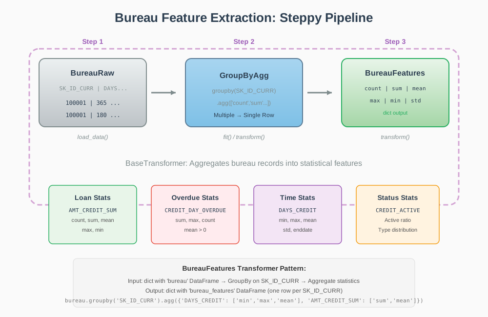
这个数据集的核心特征工程难点来自关系结构:同一客户在征信、历史申请和还款等附属表中拥有多条记录,而预测模型需要每位客户对应一个固定维度的特征向量。
示例:
 1
 2
 3
 4
 5
 6
 7
 8
 9
10
11
12
13
| Client A - Bureau Records:
├─ Record 1: SK_ID_BUREAU=101, AMT_CREDIT_SUM=5000, DAYS_CREDIT=-365
├─ Record 2: SK_ID_BUREAU=102, AMT_CREDIT_SUM=3000, DAYS_CREDIT=-180
├─ Record 3: SK_ID_BUREAU=103, AMT_CREDIT_SUM=8000, DAYS_CREDIT=-90
└─ Record 4: SK_ID_BUREAU=104, AMT_CREDIT_SUM=2000, DAYS_CREDIT=-30
Required Transformation (Single Row):
- bureau_count: 4
- bureau_amt_sum: 18000
- bureau_amt_mean: 4500
- bureau_amt_max: 8000
- bureau_days_min: -365
- bureau_days_max: -30
|
5.2 聚合方法#
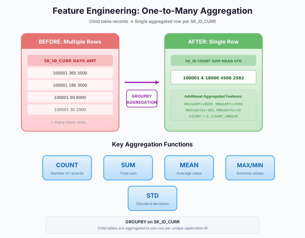
聚合算子:
| 算子 | 数学定义 | 使用场景 | 业务含义 |
|---|
| COUNT | \(n = |{r_1, r_2, …, r_n}|\) | 记录频次 | 贷款或申请次数 |
| SUM | \(\Sigma = \sum_{i=1}^{n} x_i\) | 总敞口 | 累计债务、总还款额 |
| MEAN | \(\mu = \frac{1}{n}\sum_{i=1}^{n} x_i\) | 集中趋势 | 平均贷款金额 |
| MEDIAN | \(\tilde{x} = Q_2(x)\) | 稳健的集中趋势 | 收入中位数,对异常值较稳健 |
| MAX/MIN | \(\max(x), \min(x)\) | 极值 | 最大贷款、最早记录 |
| STD | \(\sigma = \sqrt{\frac{1}{n}\sum_{i=1}^{n}(x_i - \mu)^2}\) | 波动程度 | 收入稳定性、还款一致性 |
| NUNIQUE | \(|{x_1, x_2, …}|\) | 不同值的数量 | 不同放贷机构的数量 |
5.3 各数据表的特征提取#
5.3.1 征信特征工程#
 1
 2
 3
 4
 5
 6
 7
 8
 9
10
11
12
13
14
15
16
17
18
19
20
21
22
23
24
25
26
27
28
29
30
31
32
33
34
35
36
37
38
39
40
41
42
43
44
45
| class BureauFeatureExtractor(BaseTransformer):
"""
Extracts aggregated features from credit bureau records.
"""
def transform(self, bureau: pd.DataFrame) -> Dict[str, pd.DataFrame]:
# Primary aggregations
bureau_agg = bureau.groupby('SK_ID_CURR').agg({
# Exposure metrics
'SK_ID_BUREAU': 'count',
'AMT_CREDIT_SUM': ['sum', 'mean', 'max', 'min', 'std'],
'AMT_CREDIT_SUM_DEBT': ['sum', 'mean', 'max'],
'AMT_CREDIT_SUM_OVERDUE': ['sum', 'mean', 'max'],
# Delinquency metrics
'CNT_CREDIT_PROLONG': ['sum', 'mean'],
'CREDIT_DAY_OVERDUE': ['sum', 'max', 'mean'],
# Temporal metrics
'DAYS_CREDIT': ['min', 'max', 'mean'],
'DAYS_CREDIT_ENDDATE': ['min', 'max'],
'DAYS_CREDIT_UPDATE': ['min', 'max'],
})
# Flatten multi-level columns
bureau_agg.columns = [
'_'.join(col).strip()
for col in bureau_agg.columns.values
]
# Active credit subset analysis
active_mask = bureau['CREDIT_ACTIVE'] == 'Active'
active_loans = bureau[active_mask].groupby('SK_ID_CURR').agg({
'AMT_CREDIT_SUM': ['sum', 'count'],
'AMT_CREDIT_SUM_DEBT': 'sum',
})
active_loans.columns = [
'bureau_active_' + '_'.join(col)
for col in active_loans.columns
]
# Combine feature sets
features = bureau_agg.join(active_loans, how='left')
return {'bureau_features': features}
|
生成特征示例:
 1
 2
 3
 4
 5
 6
 7
 8
 9
10
| {
'SK_ID_BUREAU_count': 5, # Total credit relationships
'AMT_CREDIT_SUM_sum': 45000, # Total credit exposure
'AMT_CREDIT_SUM_mean': 9000, # Average loan size
'AMT_CREDIT_SUM_max': 20000, # Maximum single exposure
'DAYS_CREDIT_min': -730, # Oldest relationship
'DAYS_CREDIT_max': -30, # Most recent relationship
'bureau_active_AMT_CREDIT_SUM_sum': 15000, # Active exposure
'bureau_active_SK_ID_BUREAU_count': 2, # Number of active accounts
}
|
5.3.2 历史申请特征工程#
 1
 2
 3
 4
 5
 6
 7
 8
 9
10
11
12
13
14
15
16
17
18
19
20
21
22
23
24
25
26
27
28
29
30
31
32
33
34
35
36
37
38
39
40
41
42
43
44
45
46
47
48
49
| class PreviousApplicationFeatureExtractor(BaseTransformer):
"""
Extracts features from historical Home Credit applications.
"""
def transform(self, prev_app: pd.DataFrame) -> Dict[str, pd.DataFrame]:
# Core aggregations
prev_agg = prev_app.groupby('SK_ID_CURR').agg({
# Application frequency
'SK_ID_PREV': 'count',
# Approval metrics
'NAME_CONTRACT_STATUS': [
lambda x: (x == 'Approved').sum(),
lambda x: (x == 'Refused').sum(),
lambda x: (x == 'Canceled').sum()
],
# Financial metrics
'AMT_APPLICATION': ['sum', 'mean', 'max', 'min'],
'AMT_CREDIT': ['sum', 'mean', 'max'],
'AMT_DOWN_PAYMENT': ['sum', 'mean'],
'AMT_ANNUITY': ['mean', 'max'],
# Pricing metrics
'RATE_INTEREST_PRIMARY': ['mean', 'max'],
'RATE_DOWN_PAYMENT': ['mean', 'max'],
# Temporal metrics
'DAYS_DECISION': ['min', 'max', 'mean'],
})
# Derived metrics
total_apps = prev_agg[('SK_ID_PREV', 'count')]
approved_apps = prev_agg[('NAME_CONTRACT_STATUS', '<lambda_0>')]
prev_agg['approval_rate'] = approved_apps / total_apps
prev_agg['credit_to_application_ratio'] = (
prev_agg[('AMT_CREDIT', 'sum')] /
prev_agg[('AMT_APPLICATION', 'sum')]
)
# Flatten column structure
prev_agg.columns = [
'_'.join(col).strip() if isinstance(col, tuple) else col
for col in prev_agg.columns
]
return {'previous_application_features': prev_agg}
|
关键衍生特征:
approval_rate:历史获批概率。credit_to_application_ratio:获批金额与申请金额的比率。avg_down_payment_rate:典型首付行为。
5.3.3 分期还款特征工程#
 1
 2
 3
 4
 5
 6
 7
 8
 9
10
11
12
13
14
15
16
17
18
19
20
21
22
23
24
25
26
27
28
29
30
31
32
33
34
35
36
37
38
39
40
| class InstallmentFeatureExtractor(BaseTransformer):
"""
Extracts repayment behavior features from installment records.
"""
def transform(self, installments: pd.DataFrame) -> Dict[str, pd.DataFrame]:
# Calculate derived metrics
installments['DPD'] = (
installments['DAYS_ENTRY_PAYMENT'] -
installments['DAYS_INSTALMENT']
)
installments['AMT_DIFF'] = (
installments['AMT_PAYMENT'] -
installments['AMT_INSTALMENT']
)
# Aggregations
install_agg = installments.groupby('SK_ID_CURR').agg({
# Volume metrics
'NUM_INSTALMENT_VERSION': 'count',
# Delinquency metrics
'DPD': ['mean', 'max', 'sum', lambda x: (x > 0).sum()],
# Payment amount metrics
'AMT_INSTALMENT': ['sum', 'mean', 'max'],
'AMT_PAYMENT': ['sum', 'mean', 'max'],
'AMT_DIFF': [
'mean', 'sum', 'max', 'min',
lambda x: (x > 0).sum()
],
})
# Flatten columns
install_agg.columns = [
'_'.join(col).strip()
for col in install_agg.columns.values
]
return {'installment_features': install_agg}
|
关键衍生指标:
DPD_mean:平均逾期天数。DPD_max:最严重的一次逾期。AMT_DIFF_mean:平均还款金额偏差,反映多还或少还。
5.4 时间窗口特征#
假设:近期行为比历史平均水平包含更强的预测信号。
 1
 2
 3
 4
 5
 6
 7
 8
 9
10
11
12
13
14
15
16
17
18
19
20
21
22
23
24
25
26
27
28
29
30
31
32
33
34
| class TemporalWindowFeatureExtractor(BaseTransformer):
"""
Extracts time-windowed aggregations for trend analysis.
"""
def transform(
self,
data: pd.DataFrame,
time_col: str = 'MONTHS_BALANCE'
) -> Dict[str, pd.DataFrame]:
window_sizes = [3, 6, 12, 24] # months
all_features = {}
for window in window_sizes:
# Subset to recent history
recent_mask = data[time_col] >= -window
recent_data = data[recent_mask]
# Window-specific aggregations
window_agg = recent_data.groupby('SK_ID_CURR').agg({
'AMT_BALANCE': ['mean', 'max', 'sum'],
'SK_ID_PREV': 'count',
})
# Rename with window suffix
window_agg.columns = [
f'{col}_last_{window}m'
for col in window_agg.columns
]
all_features[f'window_{window}m'] = window_agg
return all_features
|
5.5 类别变量编码#
编码策略选择:
| 方法 | 适用情况 | 优点 | 缺点 |
|---|
| 标签编码 | 有序类别,如教育水平 | 简单、维度低 | 对无序类别引入虚假顺序 |
| 独热编码 | 低基数无序类别,如性别 | 不假设类别有序 | 可能导致维度膨胀 |
| 目标编码 | 高基数类别,如职业、地区 | 捕捉与目标的关系 | 存在过拟合风险 |
| 频率编码 | 高基数标识符 | 简单,可反映出现频率 | 存在信息损失 |
实现:
 1
 2
 3
 4
 5
 6
 7
 8
 9
10
11
12
13
14
15
16
17
18
19
20
21
22
23
24
25
26
27
28
29
30
31
| from category_encoders import TargetEncoder, OneHotEncoder
class CategoricalEncodingPipeline(BaseTransformer):
"""
Applies appropriate encoding strategies by variable type.
"""
def __init__(self):
self.encoders = {}
def fit(self, X: pd.DataFrame, y: pd.Series):
# Target encoding for high-cardinality features
high_cardinality = [
'OCCUPATION_TYPE', 'ORGANIZATION_TYPE',
'NAME_FAMILY_STATUS'
]
for col in high_cardinality:
encoder = TargetEncoder(cols=[col], smoothing=10.0)
encoder.fit(X[[col]], y)
self.encoders[col] = encoder
return self
def transform(self, X: pd.DataFrame) -> Dict[str, pd.DataFrame]:
X_encoded = X.copy()
for col, encoder in self.encoders.items():
X_encoded[col] = encoder.transform(X[[col]])
return {'features_encoded': X_encoded}
|
5.6 特征选择#
目标:降低维度、消除噪声、提高训练效率。
 1
 2
 3
 4
 5
 6
 7
 8
 9
10
11
12
13
14
15
16
17
18
19
20
21
22
23
24
25
26
27
28
| from sklearn.feature_selection import mutual_info_classif, SelectKBest
class FeatureSelectionTransformer(BaseTransformer):
"""
Selects top-K features based on mutual information.
"""
def __init__(self, k: int = 500):
self.k = k
self.selector = None
def fit(self, X: pd.DataFrame, y: pd.Series):
self.selector = SelectKBest(
score_func=mutual_info_classif,
k=self.k
)
self.selector.fit(X, y)
self.selected_features = X.columns[
self.selector.get_support()
].tolist()
return self
def transform(self, X: pd.DataFrame) -> Dict[str, pd.DataFrame]:
X_selected = X[self.selected_features]
return {
'features': X_selected,
'feature_names': self.selected_features
}
|
6. 模型选择、训练与评估#
6.1 梯度提升决策树#
理论基础:
梯度提升通过函数空间中的梯度下降,构建弱学习器(通常为决策树)的加性集成:
\[F_m(x) = F_{m-1}(x) + \nu \cdot h_m(x)\]
其中,$h_m(x)$ 是针对伪残差拟合的弱学习器:
\[r_{im} = -\left[\frac{\partial L(y_i, F(x_i))}{\partial F(x_i)}\right]_{F=F_{m-1}}\]
处理表格数据的优势:
- 自动建模特征交互:树分裂天然能够表示特征组合。
- 缺失值处理:原生支持缺失值,无需预先填补。
- 非线性表达能力:捕捉复杂的决策边界。
- 可解释性:支持特征重要性和部分依赖分析。
6.2 LightGBM、XGBoost 与 CatBoost 对比#
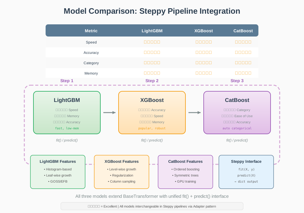
算法特性:
| 特性 | LightGBM | XGBoost | CatBoost |
|---|
| 树生长方式 | 按叶生长 | 按层生长 | 按层生长 |
| 分裂点搜索 | 基于直方图 | 直方图 + 精确搜索 | 对称树 |
| 关键优化 | GOSS、EFB | 缓存感知访问 | 有序提升 |
| 类别特征支持 | 有限支持 | 手动编码 | 原生支持 |
| 训练速度 | 最快 | 中等 | 中等 |
| 内存效率 | 最优 | 中等 | 良好 |
基于梯度的单边采样(GOSS):LightGBM
保留梯度较大、误差较高的样本,同时随机抽取小梯度样本,在维持数据分布的同时加快训练。
互斥特征捆绑(EFB):LightGBM
将很少同时为非零值的互斥特征捆绑,在不丢失信息的前提下降低维度。
有序提升(Ordered Boosting):CatBoost
通过训练数据的有序排列消除预测偏移,提供无偏梯度估计。
选择建议:
- 快速实验:LightGBM,具有 10 倍训练速度优势。
- 追求最高准确性:XGBoost,提升幅度较小但较稳定。
- 类别数据丰富:CatBoost,原生处理类别特征。
6.3 LightGBM 实现#
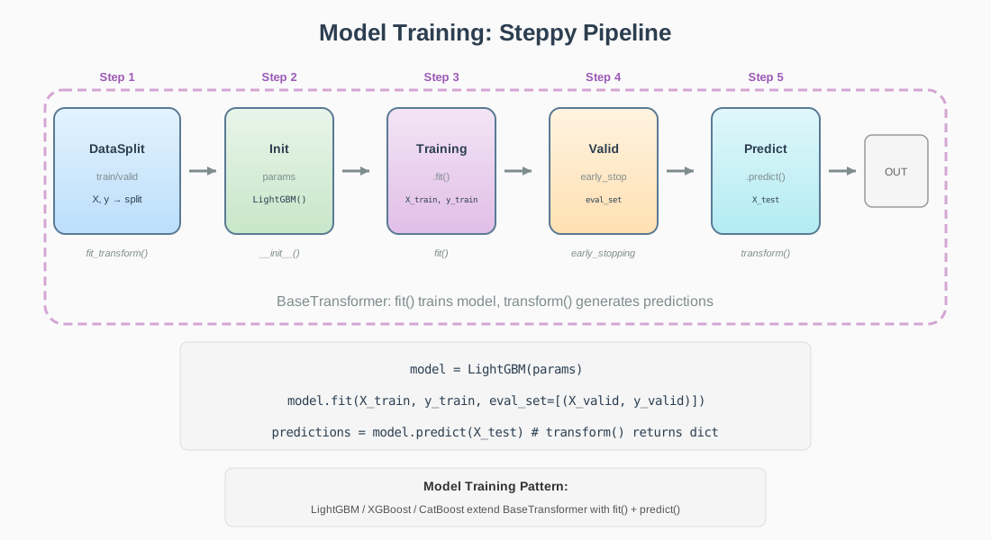
超参数配置:
 1
 2
 3
 4
 5
 6
 7
 8
 9
10
11
12
13
14
15
16
17
18
19
20
21
22
23
24
25
26
27
28
29
30
31
| import lightgbm as lgb
# Model configuration
LGBM_PARAMS = {
'objective': 'binary',
'metric': 'auc',
'boosting_type': 'gbdt',
# Tree structure
'num_leaves': 35,
'max_depth': -1,
'min_child_samples': 70,
# Learning dynamics
'learning_rate': 0.02,
'n_estimators': 5000,
# Regularization
'reg_lambda': 100.0,
'reg_alpha': 0.0,
# Sampling
'subsample': 1.0,
'colsample_bytree': 0.03,
# Categorical handling
'categorical_feature': 'auto',
'verbose': -1,
'random_state': 42
}
|
训练过程:
 1
 2
 3
 4
 5
 6
 7
 8
 9
10
11
12
13
14
15
16
17
18
19
20
21
22
23
24
25
26
27
28
29
30
31
32
33
34
35
36
37
38
39
40
41
42
| from sklearn.model_selection import train_test_split
from sklearn.metrics import roc_auc_score
# Data preparation
X_train, X_valid, y_train, y_valid = train_test_split(
X, y,
test_size=0.2,
stratify=y,
random_state=42
)
# Dataset construction
train_dataset = lgb.Dataset(X_train, label=y_train)
valid_dataset = lgb.Dataset(X_valid, label=y_valid, reference=train_dataset)
# Model training
model = lgb.train(
LGBM_PARAMS,
train_dataset,
num_boost_round=5000,
valid_sets=[train_dataset, valid_dataset],
valid_names=['train', 'valid'],
callbacks=[
lgb.early_stopping(stopping_rounds=100),
lgb.log_evaluation(period=100)
]
)
# Performance evaluation
y_pred = model.predict(X_valid, num_iteration=model.best_iteration)
validation_auc = roc_auc_score(y_valid, y_pred)
print(f'Validation AUC: {validation_auc:.4f}')
# Feature importance analysis
importance_df = pd.DataFrame({
'feature': model.feature_name(),
'importance_gain': model.feature_importance(importance_type='gain'),
'importance_split': model.feature_importance(importance_type='split')
}).sort_values('importance_gain', ascending=False)
print("\nTop 20 Features by Gain:")
print(importance_df.head(20))
|
超参数调整建议:
num_leaves:以 \(2^{\text{max\_depth}}\) 为参考基准,适当降低以控制过拟合。learning_rate:通常在 0.01—0.1 范围内,较低的值需要更多迭代。reg_lambda:对于噪声较多的数据,可从 1 增至 100。colsample_bytree:对于高维特征,可从 1.0 降至 0.3。
6.4 XGBoost 实现#
 1
 2
 3
 4
 5
 6
 7
 8
 9
10
11
12
13
14
15
16
17
18
19
20
21
22
23
24
25
26
27
28
29
30
31
32
33
34
| import xgboost as xgb
XGB_PARAMS = {
'objective': 'binary:logistic',
'eval_metric': 'auc',
'max_depth': 6,
'learning_rate': 0.05,
'subsample': 0.8,
'colsample_bytree': 0.8,
'reg_alpha': 0.1,
'reg_lambda': 1.0,
'tree_method': 'hist',
'seed': 42
}
# DMatrix construction
dtrain = xgb.DMatrix(X_train, label=y_train, enable_categorical=True)
dvalid = xgb.DMatrix(X_valid, label=y_valid, enable_categorical=True)
# Training
eval_results = {}
model = xgb.train(
XGB_PARAMS,
dtrain,
num_boost_round=1000,
evals=[(dtrain, 'train'), (dvalid, 'valid')],
evals_result=eval_results,
early_stopping_rounds=100,
verbose_eval=100
)
# Evaluation
y_pred = model.predict(dvalid)
auc = roc_auc_score(y_valid, y_pred)
|
6.5 CatBoost 实现#
 1
 2
 3
 4
 5
 6
 7
 8
 9
10
11
12
13
14
15
16
17
18
19
20
21
22
23
24
25
26
27
28
29
| from catboost import CatBoostClassifier, Pool
# Identify categorical features
categorical_features = [
i for i, col in enumerate(X_train.columns)
if X_train[col].dtype == 'object'
]
# Data pools
train_pool = Pool(X_train, y_train, cat_features=categorical_features)
valid_pool = Pool(X_valid, y_valid, cat_features=categorical_features)
# Model configuration
model = CatBoostClassifier(
iterations=1000,
learning_rate=0.05,
depth=6,
l2_leaf_reg=3.0,
early_stopping_rounds=100,
verbose=100,
random_seed=42
)
# Training
model.fit(train_pool, eval_set=valid_pool)
# Evaluation
y_pred = model.predict_proba(valid_pool)[:, 1]
auc = roc_auc_score(y_valid, y_pred)
|
6.6 交叉验证与折外预测#
使用交叉验证的原因:
- 稳定性评估:降低单次训练集与测试集划分带来的方差。
- 防止过拟合:验证模型的泛化能力。
- 生成 OOF:为模型集成提供无偏的折外预测。
分层 K 折实现:
 1
 2
 3
 4
 5
 6
 7
 8
 9
10
11
12
13
14
15
16
17
18
19
20
21
22
23
24
25
26
27
28
29
30
31
32
33
34
35
36
37
38
| from sklearn.model_selection import StratifiedKFold
N_FOLDS = 5
kf = StratifiedKFold(n_splits=N_FOLDS, shuffle=True, random_state=42)
oof_predictions = np.zeros(len(X_train))
test_predictions = np.zeros(len(X_test))
fold_scores = []
for fold, (train_idx, valid_idx) in enumerate(kf.split(X_train, y_train)):
print(f'\nFold {fold + 1}/{N_FOLDS}')
# Data partitioning
X_tr, X_val = X_train.iloc[train_idx], X_train.iloc[valid_idx]
y_tr, y_val = y_train.iloc[train_idx], y_train.iloc[valid_idx]
# Model training
model = lgb.LGBMClassifier(**LGBM_PARAMS)
model.fit(
X_tr, y_tr,
eval_set=[(X_val, y_val)],
callbacks=[lgb.early_stopping(100), lgb.log_evaluation(0)]
)
# Out-of-fold predictions
oof_predictions[valid_idx] = model.predict_proba(X_val)[:, 1]
# Test set predictions (ensemble across folds)
test_predictions += model.predict_proba(X_test)[:, 1] / N_FOLDS
# Fold-level evaluation
fold_auc = roc_auc_score(y_val, oof_predictions[valid_idx])
fold_scores.append(fold_auc)
print(f'Fold AUC: {fold_auc:.4f}')
# Aggregate performance
overall_auc = roc_auc_score(y_train, oof_predictions)
print(f'\nOverall OOF AUC: {overall_auc:.4f} (+/- {np.std(fold_scores):.4f})')
|
7. 集成学习与模型融合#
7.1 集成学习理论#
单模型的局限:
不同模型存在各自的不足:
- LightGBM:容易在稀疏特征上过拟合。
- XGBoost:训练计算成本较高。
- CatBoost:为获得稳健性,可能牺牲少量准确性。
集成的优势:
- 降低方差:平均预测有助于减少波动。
- 降低偏差:不同模型捕捉互补模式。
- 稳定性:减轻单个模型失效的影响。
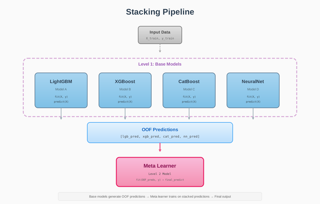
7.2 两层堆叠架构#
架构说明:
第 1 层:基学习器,采用不同的梯度提升实现。
- LightGBM:按叶优化。
- XGBoost:按层生长,使用精确贪心算法。
- CatBoost:有序提升。
第 2 层:元学习器,采用简单的线性模型。
- 逻辑回归或岭回归。
- 原因:基学习器已提取充分信号,复杂的元学习器可能过拟合。
7.3 折外预测的生成#
关键约束:训练元学习器所用的预测,必须来自未使用该目标样本训练的基模型,以防止数据泄漏。
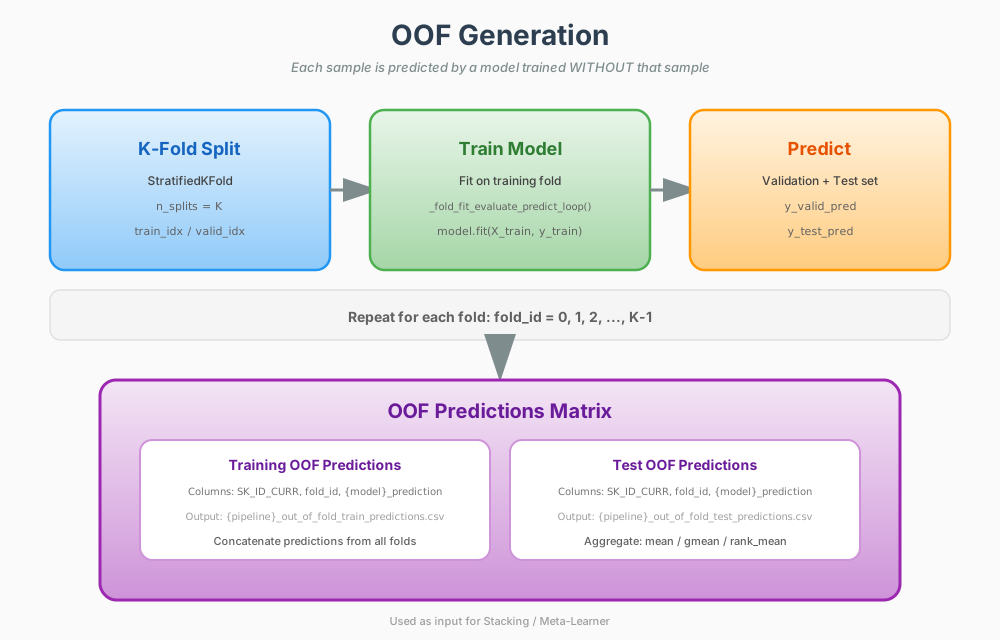
数据泄漏提醒:
1
2
3
| # INCORRECT: Training set predictions (data leakage)
model.fit(X_train, y_train)
train_pred = model.predict(X_train) # Model has seen these instances!
|
正确生成 OOF:
 1
 2
 3
 4
 5
 6
 7
 8
 9
10
11
12
| from sklearn.model_selection import StratifiedKFold
kf = StratifiedKFold(n_splits=5, shuffle=True, random_state=42)
oof_preds = np.zeros(len(X_train))
for train_idx, valid_idx in kf.split(X_train, y_train):
X_tr, X_val = X_train[train_idx], X_train[valid_idx]
y_tr = y_train[train_idx]
model.fit(X_tr, y_tr)
# Predict on held-out validation set only
oof_preds[valid_idx] = model.predict_proba(X_val)[:, 1]
|
7.4 Stacking 实现#
 1
 2
 3
 4
 5
 6
 7
 8
 9
10
11
12
13
14
15
16
17
18
19
20
21
22
23
24
25
26
27
28
29
30
31
32
33
34
35
36
37
38
39
40
41
42
43
44
45
46
47
48
49
50
51
52
53
54
55
56
57
58
59
60
61
62
63
64
65
66
67
68
69
70
71
72
73
74
75
76
77
78
79
80
81
82
83
84
85
86
87
88
89
90
91
92
93
94
95
96
| from sklearn.linear_model import LogisticRegression
from typing import Dict, Tuple
class StackingEnsemble:
"""
Two-level stacking ensemble with OOF prediction generation.
"""
def __init__(
self,
base_models: Dict[str, object],
meta_learner: object
):
self.base_models = base_models
self.meta_learner = meta_learner
self.base_predictions = {}
def fit(
self,
X: pd.DataFrame,
y: pd.Series,
cv: int = 5
) -> 'StackingEnsemble':
"""
Generate OOF predictions and train meta-learner.
"""
kf = StratifiedKFold(
n_splits=cv,
shuffle=True,
random_state=42
)
# Matrix to store OOF predictions
n_models = len(self.base_models)
oof_features = np.zeros((len(X), n_models))
# Generate OOF predictions for each base model
for idx, (name, model) in enumerate(self.base_models.items()):
print(f'Generating OOF predictions: {name}...')
for train_idx, valid_idx in kf.split(X, y):
X_tr = X.iloc[train_idx]
X_val = X.iloc[valid_idx]
y_tr = y.iloc[train_idx]
# Fit on training fold
model.fit(X_tr, y_tr)
# Predict on validation fold
oof_features[valid_idx, idx] = (
model.predict_proba(X_val)[:, 1]
)
self.base_predictions[name] = oof_features[:, idx].copy()
# Train meta-learner on OOF features
print('Training meta-learner...')
self.meta_learner.fit(oof_features, y)
# Retrain base models on full dataset
print('Retraining base models on full data...')
for name, model in self.base_models.items():
model.fit(X, y)
return self
def predict(self, X: pd.DataFrame) -> np.ndarray:
"""
Generate ensemble predictions.
"""
# Generate base model predictions
n_models = len(self.base_models)
base_features = np.zeros((len(X), n_models))
for idx, (name, model) in enumerate(self.base_models.items()):
base_features[:, idx] = model.predict_proba(X)[:, 1]
# Meta-learner prediction
return self.meta_learner.predict_proba(base_features)[:, 1]
# Usage
base_models = {
'lightgbm': lgb.LGBMClassifier(**lgb_params),
'xgboost': xgb.XGBClassifier(**xgb_params),
'catboost': CatBoostClassifier(**ctb_params, verbose=0)
}
meta_model = LogisticRegression(
C=1.0,
solver='lbfgs',
max_iter=1000
)
ensemble = StackingEnsemble(base_models, meta_model)
ensemble.fit(X_train, y_train)
final_predictions = ensemble.predict(X_test)
|
7.5 超参数优化#
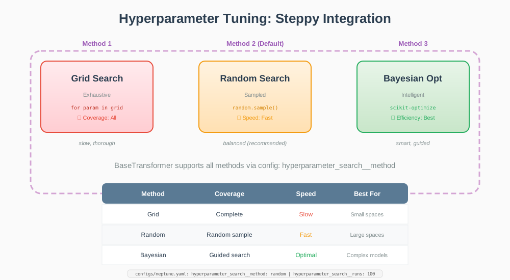
方法对比:
| 方法 | 策略 | 优势 | 局限 | 计算成本 |
|---|
| 网格搜索 | 穷举所有组合 | 覆盖全面 | 规模呈指数增长 | 高 |
| 随机搜索 | 随机采样 | 探索效率较高 | 可能遗漏较优组合 | 中等 |
| 贝叶斯优化 | 概率代理模型 | 样本利用效率高 | 实现较复杂 | 低至中等 |
贝叶斯优化实现:
 1
 2
 3
 4
 5
 6
 7
 8
 9
10
11
12
13
14
15
16
17
18
19
20
21
22
23
24
25
26
27
28
29
30
31
32
33
34
35
| from skopt import BayesSearchCV
from skopt.space import Real, Integer
# Define search space
search_spaces = {
'num_leaves': Integer(20, 50),
'learning_rate': Real(0.01, 0.1, prior='log-uniform'),
'min_child_samples': Integer(10, 100),
'reg_lambda': Real(1e-8, 10.0, prior='log-uniform'),
'subsample': Real(0.5, 1.0),
'colsample_bytree': Real(0.3, 1.0)
}
# Bayesian optimization
opt = BayesSearchCV(
lgb.LGBMClassifier(
objective='binary',
metric='auc',
boosting_type='gbdt',
n_estimators=1000,
verbose=-1
),
search_spaces,
n_iter=50,
scoring='roc_auc',
cv=3,
n_jobs=-1,
random_state=42,
verbose=1
)
opt.fit(X_train, y_train)
print(f'Best CV Score: {opt.best_score_:.4f}')
print(f'Optimal Parameters: {opt.best_params_}')
|
7.6 性能汇总#
| 模型配置 | 交叉验证 AUC | 公开排行榜 | 私有排行榜 | 相对提升 |
|---|
| LightGBM(单模型) | 0.7902 | 0.791 | 0.792 | 基线 |
| XGBoost(单模型) | 0.7854 | 0.787 | 0.788 | -0.004 |
| CatBoost(单模型) | 0.7881 | 0.789 | 0.790 | -0.002 |
| 简单平均 | 0.7920 | 0.793 | 0.794 | +0.002 |
| Stacking(LGB+XGB+CTB+LR) | 0.8053 | 0.807 | 0.808 | +0.016 |
主要认识:
- 堆叠集成相对最佳单模型提升了 1.6 个百分点。
- 在 Kaggle 排行榜中,AUC 提升 0.01 往往对应数百名的排名变化。
- 简单的逻辑回归元学习器通过减少过拟合,优于更复杂的替代方案。
8. 结论与最佳实践#
8.1 完整技术流程回顾#
 1
 2
 3
 4
 5
 6
 7
 8
 9
10
11
12
13
14
15
16
17
18
19
20
21
22
23
24
| Raw Data (7 tables, 50M+ records)
↓
Data Preprocessing
├─ Anomaly detection and treatment
├─ Missing value imputation
└─ Categorical encoding
↓
Feature Engineering (1,000+ features)
├─ Aggregation operations (count/sum/mean/max/std)
├─ Temporal window features (3m/6m/12m/24m)
├─ Ratio and interaction features
└─ Target encoding for high-cardinality variables
↓
Model Development
├─ LightGBM (primary model)
├─ XGBoost (accuracy complement)
└─ CatBoost (robustness validation)
↓
Ensemble Construction
├─ Out-of-fold prediction generation
├─ Meta-learner training
└─ Final prediction aggregation
↓
Submission (AUC 0.808, Top 5%)
|
8.2 核心技术认识#
数据架构:
- 关系型数据库结构需要系统化的聚合策略。
- 一对多关系需要谨慎提取特征,避免信息损失。
- 时间序列比静态快照提供更丰富的信号。
特征工程:
- 领域知识从根本上决定了特征构造的可能空间。
- 均值、中位数和最大值等不同聚合函数,隐含不同的业务假设。
- 时间窗口特征比历史平均值更能捕捉行为趋势。
建模策略:
- 梯度提升仍是结构化数据预测的领先方法。
- 交叉验证兼顾稳定性评估和集成准备。
- 堆叠集成能够带来持续、显著的性能提升。
8.3 可复现的工程实践#
- 流水线架构:模块化设计便于组件测试与替换。
- 配置管理:集中管理参数,便于实验追踪。
- 开发模式:通过子采样策略(
--dev_mode)缩短迭代周期。 - 实验追踪:系统记录实验日志,避免重复计算。
8.4 后续研究方向#
短期优化:1—2 周
- 探索人工设定之外的特征交互。
- 根据验证集表现优化加权集成。
- 细化超参数搜索空间。
中期扩展:1—2 个月
- 使用深度学习提取特征,例如自编码器表示。
- 使用图神经网络对关系数据建模。
- 通过 SHAP 值分解分析模型可解释性。
长期探索:3 个月以上
- 构建在线学习系统,适应分布漂移。
- 建设用于生产模型验证的 A/B 测试框架。
- 使用联邦学习架构开展跨机构协作。
8.5 推荐资源#
官方文档:
代表性论文:
- Chen, T., & Guestrin, C. (2016). XGBoost: A Scalable Tree Boosting System. KDD.
- Ke, G., et al. (2017). LightGBM: A Highly Efficient Gradient Boosting Decision Tree. NIPS.
- Prokhorenkova, L., et al. (2018). CatBoost: Unbiased Boosting with Categorical Features. NIPS.
竞赛资源:
本文对 Home Credit Default Risk 竞赛方案的分析,展示了机器学习方法在实际信用风险评估中的系统应用。项目的价值不仅在于取得的 AUC(0.808),还体现在:
- 工程规范:流水线架构保证可复现性和可维护性。
- 以数据为中心:探索性分析直接指导特征工程决策。
- 系统优化:从单模型逐步改进为复杂集成。
基本原则:
特征工程决定理论性能上限,机器学习算法则逐步逼近这一上限。持续投入数据理解与特征构建,通常比仅调整超参数更有效。
本文的方法也可迁移到以下相关领域:
- 保险欺诈检测。
- 营销响应建模。
- 客户流失预测。
- 信用评分系统开发。
本文对 Kaggle Home Credit Default Risk 竞赛方案进行了完整技术分析。开源实现见 GitHub。